Signaling Correlations

Consider a device that has a classical input $x\in\mathcal{X}=[X]$ and classical output $y\in\mathcal{Y}=[Y]$ where $[N]:=\{1,2,\cdots,N \}$ is a finite set of positive integers. The device is assumed to be causal, i.e. the output set $\mathcal{Y}$ is computed from the input $\mathcal{X}$, however, no assumptions are made about how $\mathcal{Y}$ is computed from $\mathcal{X}$. Hence this device is regarded as a black-box and this description applies to all classical technologies as well as many quantum systems used for computation and communication. Without loss of generality, any such black-box can be described as a signaling device that transmits classical information from Alice to Bob.

Signaling Black-Box

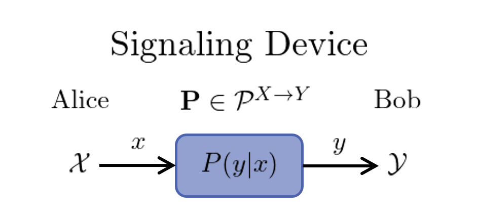
The signaling device is effectively a classical channel with $X$ inputs and $Y$ outputs, however, the signaling process that takes $\mathcal{X}\to \mathcal{Y}$ may use non-classical physics e.g. quantum physics. Making no assumptions about the physical system inside the channel, we can characterize its behavior by the conditional probabilities $P(y|x)$. We refer to these probabilities as signaling correlations and organize them into a column stochastic matrix $\mathbf{P}$ where $P(y|x)$ is the element in the $y^{th}$ row and $x^{th}$ column. Hence $\mathbf{P}$ represents a classical channel with $X$ inputs and $Y$ outputs and we denote the set of all such classical channels as $\mathcal{P}^{X\to Y}$.

The information capacity of a channel will typically be limited. In the one-shot setting, we can quantify this value by $d$, the number of distinct classical messages used. In a quantum system $d$ corresponds to the Hilbert space dimension of encoded quantum states. For example, single bit or qubit communication corresponds to $d=2$, while for general $d$ we specify a single dit or qudit of communication.

Code Example: The `LocalSignaling` Scenario

To model such signaling devices, we apply the framework of BellScenario.jl. The signaling device is then described by the BellScenario.LocalSignaling scenario which specifies the number of inputs X, outputs Y and forward communication d.

using BellScenario

X = 3    # num inputs
Y = 4    # num outputs
d = 2    # bit or qubit signaling

scenario = LocalSignaling(X, Y, d)

LocalSignaling(3, 4, 2)

Note that the constructed LocalSignaling type specifies the black-box configuration, but not whether classical or quantum signaling is used.

Classical Channels

In a classical setting, a LocalSignaling scenario decomposes as follows:

Alice (the transmitter) encodes input $x$ into a single dit message $m\in[d]$.
Message $m$ is noiselessly sent from Alice to Bob.
Bob (the receiver) decodes message $m$ to produce output $y$.

To assist in this protocol, Alice and Bob can use shared randomness to coordinate their encoding and decoding maps. This noiseless one-way communication protocol is depicted in the following image.

Classical Signaling Device

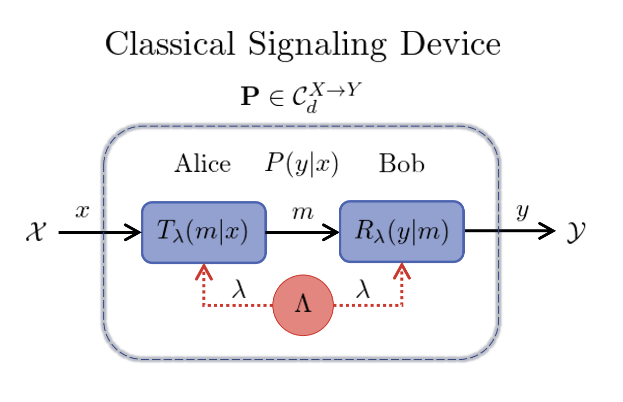
In the figure, $T_{\lambda}(m|x)$ and $R_{\lambda}(y|m)$ are the conditional probabilities for the transmitter and receiver. In fact, the transmitter and receiver can be represented as classical channels $\mathbf{T}_{\lambda}\in\mathcal{P}^{X \to d}$ and $\mathbf{R}_{\lambda} \in \mathcal{P}^{d \to Y}$. Furthermore, $\Lambda$ denotes the sample space from which shared random variable $\lambda$ is drawn with the probability $q(\lambda)$ where $\sum_{\lambda\in\Lambda} q(\lambda) = 1$. The classical signaling correlations produced in a LocalSignaling scenario decompose as

\[P(y|x) = \sum_{\lambda\in\Lambda}q(\lambda)\mathbf{R}_\lambda\mathbf{T}_\lambda = \sum_{\lambda\in\Lambda}q(\lambda) \sum_{m\in[d]}R_\lambda(y|m)T_\lambda(m|x).\]

Code Example: Classical Signaling Devices

The complete set of classical signaling correlations are denoted $\mathcal{C}_d^{X \to Y}$. Any classical channel $\mathbf{P}$ satisfies $\mathbf{P}\in\mathcal{C}_d^{X \to Y}\subset \mathcal{P}^{X \to Y}$. The set $\mathcal{C}_d^{X \to Y}$ forms a convex polytope regarded as the signaling polytope. More details on the structure of the signaling polytope are found in the Signaling Polytopes section. In the BellScenario.jl framework a classical channel $\mathbf{P}\in\mathcal{P}^{X\to Y}$ is then represented by a BellScenario.AbstractStrategy type where a Strategy is simply a column stochastic map.

Code Example: Classical Signaling without Shared Randomness

using BellScenario

X = 3    # num inputs
Y = 3    # num outputs
d = 2    # dit signaling

scenario = LocalSignaling(X, Y, d)

T = Strategy([1 0 1;0 1 0])    # transmitter channel
R = Strategy([0 0;0 1;1 0])    # receiver channel

P = *(R, T, scenario)    # `Strategy` matrix multiplication : P = R*T

3×3 Strategy:
 0.0  0.0  0.0
 0.0  1.0  0.0
 1.0  0.0  1.0

Code Example: Classical Signaling with Shared Randomness

using BellScenario

X = 3    # num inputs
Y = 3    # num outputs
d = 2    # dit signaling

scenario = LocalSignaling(X, Y, d)

# λ = 1 strategies
T1 = Strategy([1 0 1;0 1 0])    # transmitter channel 1
R1 = Strategy([0 0;0 1;1 0])    # receiver channel 1

# λ = 2 strategies
T2 = Strategy([0 0.5 1;1 0.5 0])    # transmitter channel 2
R2 = Strategy([1 0;0 1;0 0])        # receiver channel 2

Λ = [0.5, 0.5]    # shared random distribution

# `Strategy` matrix multiplication : P = R*T
P1 = *(R1, T1, scenario)
P2 = *(R2, T2, scenario)

# Convex combination of `P1` and `P2`
Strategy(sum( Λ .* [P1, P2] ), scenario)

3×3 Strategy:
 0.0  0.25  0.5
 0.5  0.75  0.0
 0.5  0.0   0.5

Quantum Channels

In a quantum setting a LocalSignaling scenario decomposes as follows:

Alice uses a classical-quantum encoder $\Psi$ to transform input $x$ into a quantum state $\rho_x$.
Alice sends $\rho_x$ to Bob through a quantum channel $\mathcal{N}$.
Bob measures $\mathcal{N}(\rho_x)$ with a positive operator-valued measure (POVM) $\Pi = \{\Pi_y\}_{y\in\mathcal{Y}}$ produce output $y$.

The amount of quantum communication is measured by the Hilbert space dimension of $\rho_x$. Additionally, the quantum channel $\mathcal{N}$ performs a completely positive trace-preserving (CPTP) map on the density matrix of $\rho_x$ producing a new quantum states $\mathcal{N}(\rho_x)$. This quantum communication scheme is depicted in the following figure.

Quantum Signaling

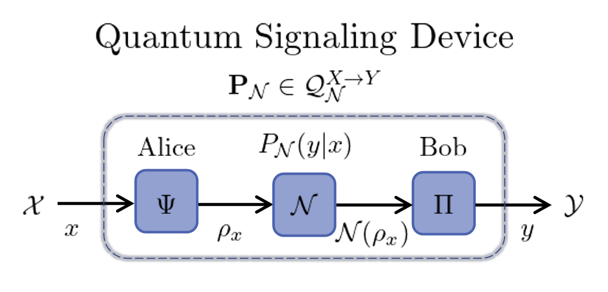
Note that the inputs and outputs are classical, hence, we discuss the classical channel $\mathbf{P}_{\mathcal{N}}$ generated using quantum channel $\mathcal{N}$. The signaling correlations of a quantum signaling device are then expressed

\[P_{\mathcal{N}}(y|x) = \text{Tr}[\Pi_y \mathcal{N}(\rho_x)],\]

for a given set of quantum states $\{\rho_x\}_{x\in\mathcal{X}}$ and POVM $\{\Pi_y\}_{y\in\mathcal{Y}}$. The set of quantum channels generated for any choice of states and POVM is denoted $\mathcal{Q}_{\mathcal{N}}^{X \to Y}$ where $\mathbf{P}_{\mathcal{N}} \in\mathcal{Q}_{\mathcal{N}}^{X \to Y}\subset \mathcal{P}^{X \to Y}$. For example, a noiseless quantum channel $\mathcal{N}=\text{id}_d$ where $\text{id}_d$ is the $d \times d$ identity matrix, the signaling correlations are constructed as

\[P_{\text{id}_d}(y|x) = \text{Tr}[\Pi_y \rho_x],\]

while the set of all noiseless channels is denoted $\mathcal{Q}_d^{X \to Y}$.

Code Example: Signaling Over a Quantum Channel

To numerically construct quantum signaling correlations, BellScenario.jl provides a quantum_strategy method. As input this method requires states and POVMs to be represented by QBase.States.AbstractDensityMatrix and QBase.Observables.AbstractPOVM as defined in the QBase.jl package.

using BellScenario
using QBase

X = 3    # num inputs
Y = 3    # num outputs
d = 2    # qudit signaling

scenario = LocalSignaling(X, Y, d)

Ψ = States.trine_qubits             # trine qubit states
Π = Observables.trine_qubit_povm    # trine qubit povm
println("Π = ", Π, "\n")

# quantum signaling correlations for an ideal channel
P = quantum_strategy(Π, Ψ, scenario)

# quantum signaling correlations for a depolarizing channel
μ = 0.5    # depolarization amount 0 ≤ μ ≤ 1
P_N = quantum_strategy(Π, Channels.depolarizing.(Ψ, μ), scenario)

Ψ = QBase.States.Qubit[[1.0 + 0.0im 0.0 + 0.0im; 0.0 + 0.0im 0.0 + 0.0im], [0.25 + 0.0im 0.4330127018922193 + 0.0im; 0.4330127018922193 + 0.0im 0.7499999999999999 + 0.0im], [0.25 + 0.0im -0.4330127018922193 - 0.0im; -0.4330127018922193 + 0.0im 0.7499999999999999 + 0.0im]]

Π = Array{Complex{Float64},2}[[0.6666666666666666 + 0.0im 0.0 + 0.0im; 0.0 + 0.0im 0.0 + 0.0im], [0.16666666666666666 + 0.0im 0.28867513459481287 + 0.0im; 0.28867513459481287 + 0.0im 0.4999999999999999 + 0.0im], [0.16666666666666666 + 0.0im -0.28867513459481287 - 0.0im; -0.28867513459481287 + 0.0im 0.4999999999999999 + 0.0im]]

P = [0.6666666666666666 0.16666666666666666 0.16666666666666666; 0.16666666666666666 0.6666666666666665 0.16666666666666657; 0.16666666666666666 0.16666666666666657 0.6666666666666665]

P_N = [0.5 0.25 0.25; 0.24999999999999997 0.49999999999999994 0.24999999999999994; 0.24999999999999997 0.24999999999999994 0.49999999999999994]